A
low-pass filter is a filter that passes low-frequency
signals but attenuates (reduces the amplitude of) signals with frequencies higher than the cutoff frequency. The actual amount of attenuation for each frequency varies from filter to filter. It is sometimes called a
high-cut filter, or
treble cut filter when used in audio applications. A low-pass filter is the opposite of a high-pass filter, and a band-pass filter is a combination of a low-pass and a high-pass.
Low-pass filters exist in many different forms, including electronic circuits (such as a
hiss filter used in audio), digital filters for smoothing sets of data, acoustic barriers, blurring of images, and so on. The moving average operation used in fields such as finance is a particular kind of low-pass filter, and can be analyzed with the same signal processing
techniques as are used for other low-pass filters. Low-pass filters provide a smoother form of a signal, removing the short-term fluctuations, and leaving the longer-term trend
Examples of low-pass filters
Acoustic
A stiff physical barrier tends to reflect higher sound frequencies, and so acts as a low-pass filter for transmitting sound. When music is playing in another room, the low notes are easily heard, while the high notes are attenuated.
Electronic
In an electronic low-pass RC filter for voltage signals, high frequencies contained in the input signal are attenuated but the filter has little attenuation below its cutoff frequency which is determined by its RC time constant.
For current signals, a similar circuit using a resistor and capacitor in parallel works in a similar manner. See current divider discussed in more detail below.
Electronic low-pass filters are used to drive subwoofers and other types of loudspeakers, to block high pitches that they can't efficiently broadcast.
Radio transmitters use low-pass filters to block harmonic emissions which might cause interference with other communications.
The tone knob found on many electric guitars is a low-pass filter used to reduce the amount of treble in the sound.
An integrator is another example of a single time constant low-pass filter.
[1]
Telephone lines fitted with DSL splitters use low-pass and high-pass filters to separate DSL and POTS signals sharing the same pair of wires.
Low-pass filters also play a significant role in the sculpting of sound for electronic music as created by analogue synthesisers.
See subtractive synthesis.
Ideal and real filters
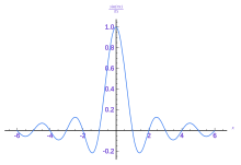
The sinc function, the impulse response of an ideal low-pass filter.
An ideal low-pass filter completely eliminates all frequencies above the cutoff frequency while passing those below unchanged: its frequency response is a rectangular function, and is a brick-wall filter. The transition region present in practical filters does not exist in an ideal filter. An ideal low-pass filter can be realized mathematically (theoretically) by multiplying a signal by the rectangular function in the frequency domain or, equivalently, convolution with its impulse response, a sinc function, in the time domain.
However, the ideal filter is impossible to realize without also having signals of infinite extent in time, and so generally needs to be approximated for real ongoing signals, because the sinc function's support region extends to all past and future times. The filter would therefore need to have infinite delay, or knowledge of the infinite future and past, in order to perform the convolution. It is effectively realizable for pre-recorded digital signals by assuming extensions of zero into the past and future, or more typically by making the signal repetitive and using Fourier analysis.
Real filters for real-time applications approximate the ideal filter by truncating and windowing the infinite impulse response to make a finite impulse response; applying that filter requires delaying the signal for a moderate period of time, allowing the computation to "see" a little bit into the future. This delay is manifested as phase shift. Greater accuracy in approximation requires a longer delay.
An ideal low-pass filter results in ringing artifacts via the Gibbs phenomenon. These can be reduced or worsened by choice of windowing function, and the design and choice of real filters involves understanding and minimizing these artifacts. For example, "simple truncation [of sinc] causes severe ringing artifacts," in signal reconstruction, and to reduce these artifacts one uses window functions "which drop off more smoothly at the edges."
[2]
The Whittaker–Shannon interpolation formula describes how to use a perfect low-pass filter to reconstruct a continuous signal from a sampled digital signal. Real digital-to-analog converters use real filter approximations.
Continuous-time low-pass filters

The gain-magnitude frequency response of a first-order (one-pole) low-pass filter.
Power gain is shown in decibels (i.e., a 3 dB decline reflects an additional half-power attenuation). Angular frequency is shown on a logarithmic scale in units of radians per second.
There are many different types of filter circuits, with different responses to changing frequency. The frequency response of a filter is generally represented using a Bode plot, and the filter is characterized by its cutoff frequency and rate of frequency rolloff. In all cases, at the
cutoff frequency, the filter attenuates the input power by half or 3 dB. So the
order of the filter determines the amount of additional attenuation for frequencies higher than the cutoff frequency.
- A first-order filter, for example, will reduce the signal amplitude by half (so power reduces by 6 dB) every time the frequency doubles (goes up one octave); more precisely, the power rolloff approaches 20 dB per decade in the limit of high frequency. The magnitude Bode plot for a first-order filter looks like a horizontal line below the cutoff frequency, and a diagonal line above the cutoff frequency. There is also a "knee curve" at the boundary between the two, which smoothly transitions between the two straight line regions. If the transfer function of a first-order low-pass filter has a zero as well as a pole, the Bode plot will flatten out again, at some maximum attenuation of high frequencies; such an effect is caused for example by a little bit of the input leaking around the one-pole filter; this one-pole–one-zero filter is still a first-order low-pass. See Pole–zero plot and RC circuit.
- A second-order filter attenuates higher frequencies more steeply. The Bode plot for this type of filter resembles that of a first-order filter, except that it falls off more quickly. For example, a second-order Butterworth filter will reduce the signal amplitude to one fourth its original level every time the frequency doubles (so power decreases by 12 dB per octave, or 40 dB per decade). Other all-pole second-order filters may roll off at different rates initially depending on their Q factor, but approach the same final rate of 12 dB per octave; as with the first-order filters, zeroes in the transfer function can change the high-frequency asymptote. See RLC circuit.
- Third- and higher-order filters are defined similarly. In general, the final rate of power rolloff for an order-n all-pole filter is 6n dB per octave (i.e., 20n dB per decade).
On any Butterworth filter, if one extends the horizontal line to the right and the diagonal line to the upper-left (the asymptotes of the function), they will intersect at exactly the "cutoff frequency". The frequency response at the cutoff frequency in a first-order filter is 3 dB below the horizontal line. The various types of filters – Butterworth filter, Chebyshev filter, Bessel filter, etc. – all have different-looking "knee curves". Many second-order filters are designed to have "peaking" or resonance, causing their frequency response at the cutoff frequency to be
above the horizontal line.
See electronic filter for other types.
The meanings of 'low' and 'high' – that is, the cutoff frequency – depend on the characteristics of the filter. The term "low-pass filter" merely refers to the shape of the filter's response; a high-pass filter could be built that cuts off at a lower frequency than any low-pass filter – it is their responses that set them apart. Electronic circuits can be devised for any desired frequency range, right up through microwave frequencies (above 1 GHz) and higher.
Laplace notation
Continuous-time filters can also be described in terms of the Laplace transform of their impulse response in a way that allows all of the characteristics of the filter to be easily analyzed by considering the pattern of poles and zeros of the Laplace transform in the complex plane (in discrete time, one can similarly consider the Z-transform of the impulse response).
For example, a first-order low-pass filter can be described in Laplace notation as

where
s is the Laplace transform variable,
τ is the filter time constant, and
K is the filter passband gain.
Electronic low-pass filters
Passive electronic realization

Passive, first order low-pass RC filter
One simple electrical circuit that will serve as a low-pass filter consists of a resistor in series with a load, and a capacitor in parallel with the load. The capacitor exhibits reactance, and blocks low-frequency signals, causing them to go through the load instead. At higher frequencies the reactance drops, and the capacitor effectively functions as a short circuit. The combination of resistance and capacitance gives you the time constant of the filter
τ = RC (represented by the Greek letter tau). The break frequency, also called the turnover frequency or cutoff frequency (in hertz), is determined by the time constant:

or equivalently (in radians per second):
One way to understand this circuit is to focus on the time the capacitor takes to charge. It takes time to charge or discharge the capacitor through that resistor:
- At low frequencies, there is plenty of time for the capacitor to charge up to practically the same voltage as the input voltage.
- At high frequencies, the capacitor only has time to charge up a small amount before the input switches direction. The output goes up and down only a small fraction of the amount the input goes up and down. At double the frequency, there's only time for it to charge up half the amount.
Another way to understand this circuit is with the idea of reactance at a particular frequency:
- Since DC cannot flow through the capacitor, DC input must "flow out" the path marked Vout (analogous to removing the capacitor).
- Since AC flows very well through the capacitor — almost as well as it flows through solid wire — AC input "flows out" through the capacitor, effectively short circuiting to ground (analogous to replacing the capacitor with just a wire).
The capacitor is not an "on/off" object (like the block or pass fluidic explanation above). The capacitor will variably act between these two extremes. It is the Bode plot and frequency response that show this variability.
Active electronic realization

An active low-pass filter
Another type of electrical circuit is an
active low-pass filter.
In the operational amplifier circuit shown in the figure, the cutoff frequency (in hertz) is defined as:
or equivalently (in radians per second):

The gain in the passband is −
R2/
R1, and the stopband drops off at −6 dB per octave as it is a first-order filter.
Sometimes, a simple gain amplifier (as opposed to the very-high-gain operational amplifier) is turned into a low-pass filter by simply adding a feedback capacitor
C. This feedback decreases the frequency response at high frequencies via the Miller effect, and helps to avoid oscillation in the amplifier. For example, an audio amplifier can be made into a low-pass filter with cutoff frequency 100 kHz to reduce gain at frequencies which would otherwise oscillate. Since the audio band (what we can hear) only goes up to 20 kHz or so, the frequencies of interest fall entirely in the passband, and the amplifier behaves the same way as far as audio is concerned.
Discrete-time realization
For another method of conversion from continuous- to discrete-time, see Bilinear transform.
The effect of a low-pass filter can be simulated on a computer by analyzing its behavior in the time domain, and then discretizing the model.
A simple low-pass RC filter
From the circuit diagram to the right, according to Kirchoff's Laws and the definition of capacitance:
-
-
-
where
Qc(t) is the charge stored in the capacitor at time
t. Substituting equation
Q into equation
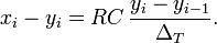
I gives

, which can be substituted into equation
V so that:

This equation can be discretized. For simplicity, assume that samples of the input and output are taken at evenly-spaced points in time separated by
ΔT time. Let the samples of
vin be represented by the sequence

, and let
vout be represented by the sequence

which correspond to the same points in time. Making these substitutions:
And rearranging terms gives the recurrence relation

That is, this discrete-time implementation of a simple RC low-pass filter is the exponentially-weighted moving average
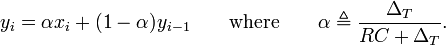
By definition, the
smoothing factor 
. The expression for
α yields the equivalent time constant
RC in terms of the sampling period
ΔT and smoothing factor
α:
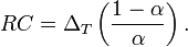
If
α = 0.5, then the
RC time constant is equal to the sampling period. If

, then
RC is significantly larger than the sampling interval, and

.
Algorithmic implementation
The filter recurrence relation provides a way to determine the output samples in terms of the input samples and the preceding output. The following pseudocode algorithm will simulate the effect of a low-pass filter on a series of digital samples:
// Return RC low-pass filter output samples, given input samples,
 // time interval dt, and time constant RC
 function lowpass(real[0..n] x, real dt, real RC)
   var real[0..n] y
   var real α := dt / (RC + dt)
   y[0] := x[0]
   for i from 1 to n
       y[i] := α * x[i] + (1-α) * y[i-1]
   return y
The loop which calculates each of the
n outputs can be refactored into the equivalent:
for i from 1 to n
       y[i] := y[i-1] + α * (x[i] - y[i-1])
That is, the change from one filter output to the next is
proportional to the difference between the previous output and the next input. This
exponential smoothing property matches the
exponential decay seen in the continuous-time system. As expected, as the
time constant RC increases, the discrete-time smoothing parameter
α decreases, and the output samples
respond more slowly to a change in the input samples
– the system will have more
inertia.